Immune receptor repertoire diversity
Tudor-Stefan Cotet, Victor Kreiner, Alexander Yermanos
09/06/2022
Source:vignettes/Diversity and sampling.Rmd
Diversity and sampling.Rmd1. Introduction
The Platypus family of packages are meant to provide potential pipelines and examples relevant to the broad field of computational immunology. The core set of functions can be found at https://github.com/alexyermanos/Platypus and examples of use can be found in the publications https://doi.org/10.1093/nargab/lqab023 and insert biorxiv database manuscript here
Stay tuned for updates https://twitter.com/AlexYermanos
Given the immense diversity encoded in adaptive immune repertoires, there has been significant progress in developing mathematical models and bioinformatic pipelines to profile and compare the sequence diversity across repertoires. This further includes metrics that can help estimate the extent to which total diversity is captured in immune repertoire sequencing experiments.
2. Loading the VGM
The output of the VDJ_GEX_matrix is the main object for all downstream functions in Platypus. We can create this directly into the R session by using the public data available on PlatypusDB. We will use the VDJ data of bone marrow plasma cells from five mice that were immunized with OVA (and the MPLA adjuvant) from Neumeier^, Yermanos^ et al 2022 PNAS.
library(Platypus)

#Currently sourcing the scripts as these functions are not in the most recent Platypus version
#source('VDJ_abundances.R')
#source('VDJ_diversity.R')
#source('VDJ_rarefaction.R')
#source('VDJ_ordination.R')

PlatypusDB_fetch(PlatypusDB.links = c("neumeier2021b//VDJmatrix"),
                                     load.to.enviroment = T, combine.objects = F)
## 2022-08-07 20:18:15: Starting download of neumeier2021b__VDJmatrix.RData...## [1] "neumeier2021b__VDJmatrix"
VDJ <- neumeier2021b__VDJmatrix[[1]]3. VDJ_abundances for feature richness plots
We will first visualize the CDRH3 and CDR species richness densities per clonotype via VDJ_abundances. This function is a flexible utility for calculating cell counts/abundances for different unique features (via the feature.columns parameter), across multiple groups (via grouping.column), and/or multiple samples (via sample.column). VDJ_abundances is used internally to get abundance data for the diversity, rarefaction, and ordination analyses, but can also be used to obtain feature barplots (output.format = ‘barplot’) or feature richness density plots (output.format = ‘density’) which we will see next. We will only plot 3 samples for better clarity.
#CDRH3 richness density plots across 3 samples
VDJ_abundances(VDJ,
               feature.columns = 'CDR3aa',
               grouping.column = 'sample_id',
               sample.column = 'none',
               output.format = 'density',
               specific.groups = c('s1','s2','s3'))
## [[1]]
#CDR3 richness density plots across 3 samples
VDJ_abundances(VDJ,
               feature.columns = 'CDR3aa',
               grouping.column = 'sample_id',
               sample.column = 'none',
               output.format = 'density',
               specific.groups = c('s1','s2','s3'))
## [[1]]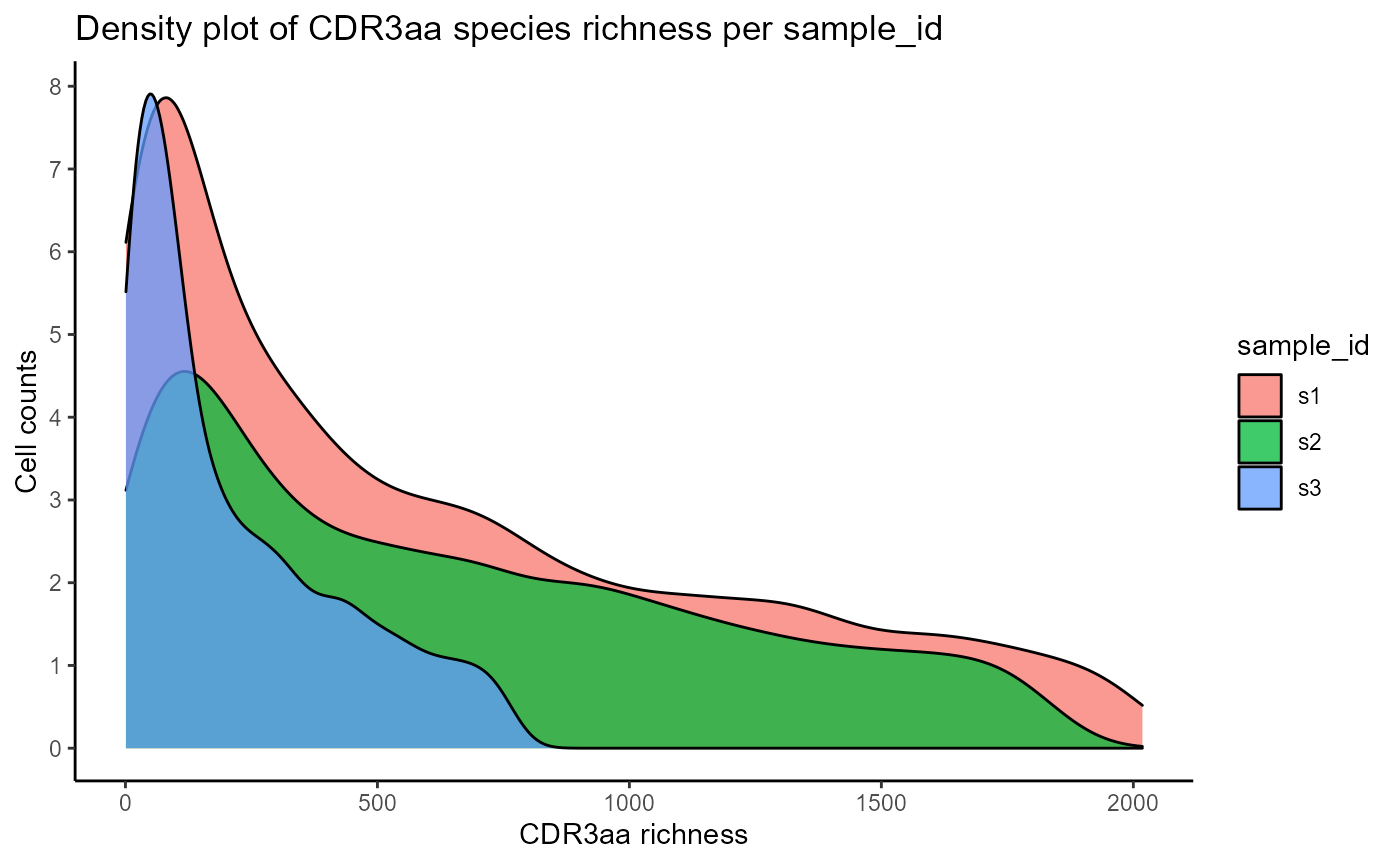
Species richness densities can also be visualized as ridgeline plots, by changing the output.format parameter to ‘density.ridges’. This requires the ggridges package.
VDJ_abundances(VDJ,
               feature.columns = 'VDJ_cdr3s_aa',
               grouping.column = 'sample_id',
               sample.column = 'none',
               output.format = 'density.ridges')
## [[1]]## Picking joint bandwidth of 50.6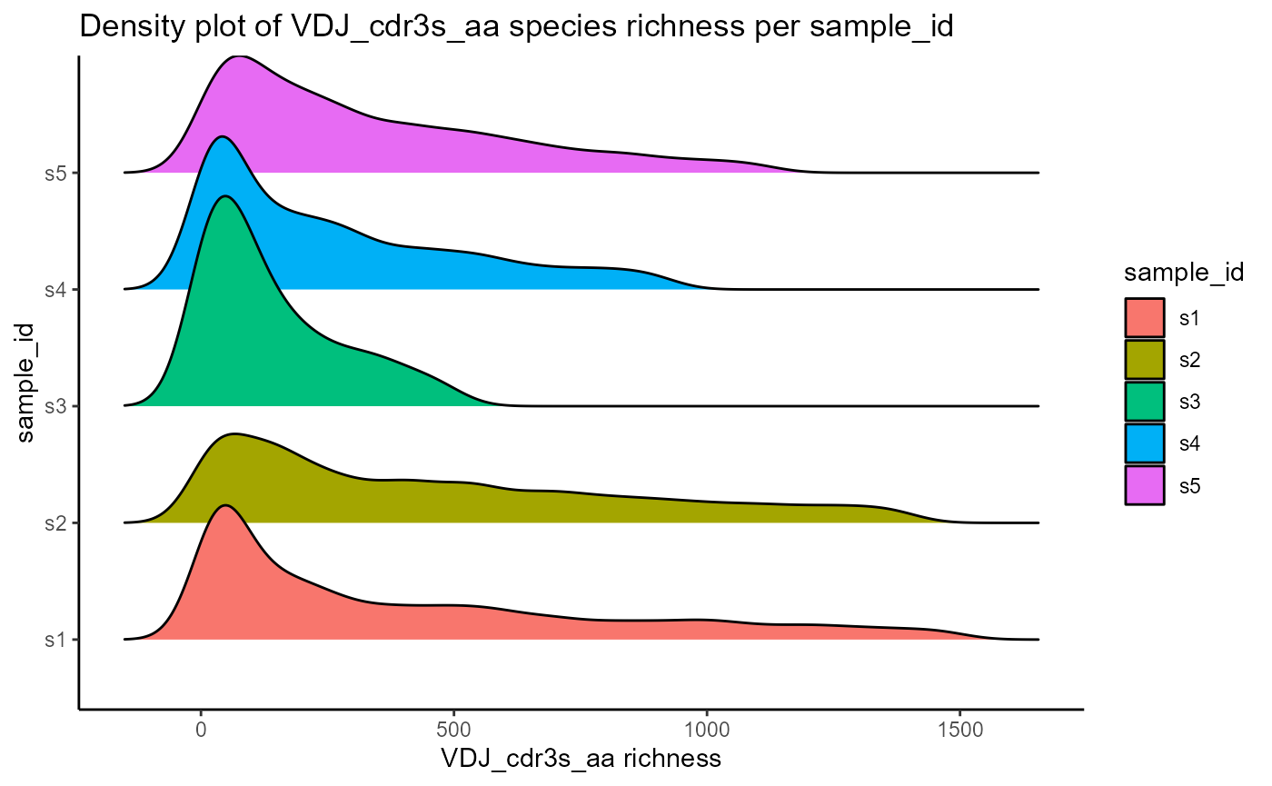
4. VDJ_diversity for α, β-diversity, and species evenness metrics
α, β-Diversity, and species evenness can be computed via VDJ_diversity.To allow flexibility, VDJ_diversity can be used to calculate diversity metrics for a wide range of features/species definitions (denoted as VDJ columns in the feature.columns parameter), across different groups (group.column parameter). We will next focus on calculating the diversity of unique CDRH3 sequences (feature.columns = ‘VDJ_cdr3s_aa’) across samples (grouping.column = ‘sample_id’).
4.1 α-Diversity
α-Diversity metrics currently implemented in VDJ_diversity include: species richness (‘richness’), the Berger-Parker index (‘bergerparker’), the Simpson index (‘simpson’), the Gini-Simpson index (‘ginisimpson’), the inverse Simpson index (‘inversesimpson’), Shannon index (‘shannon’), Chao1 (‘chao1’), ACE (‘ace’), and Good’s coverage metric (‘coverage’).
#Chao1 index for CDRH3s
VDJ_diversity(VDJ,
               feature.columns = 'VDJ_cdr3s_aa',
               grouping.column = 'sample_id',
               metric = 'chao1',
               subsample.to.same.n = T)
The parameter subsample.to.same.n allows subsampling each group to the smallest group’s size, standardizing the diversity metric across all groups for fairer comparisons. We will check the difference in species richness using subsample.to.same.n set to TRUE and then FALSE. subsample.to.same.n is set to TRUE by default for α-diversity/evenness comparisons.
#subsample.to.same.n = T
p1 <- VDJ_diversity(VDJ,
              feature.columns = 'VDJ_cdr3s_aa',
              grouping.column = 'sample_id',
              metric = 'richness',
              subsample.to.same.n = T)

#subsample.to.same.n = F
p2 <- VDJ_diversity(VDJ,
               feature.columns = 'VDJ_cdr3s_aa',
               grouping.column = 'sample_id',
               metric = 'richness',
               subsample.to.same.n = F)

cowplot::plot_grid(p1, p2)
4.2 Evenness
Evenness metrics implemented in VDJ_diversity include: the Shannon evenness index (‘shannonevenness’), Simpson evenness (‘simpsonevenness’), Bulla index (‘bulla’), Camargo index (‘camargo’), Smith-Wilson index (‘smithwilson’), and the Heip index (‘heip’).
#Simpson evenness index for CDRH3s across each sample
VDJ_diversity(VDJ,
               feature.columns = 'VDJ_cdr3s_aa',
               grouping.column = 'sample_id',
               metric = 'simpsonevenness')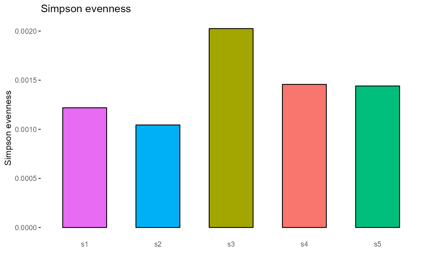
4.3 β-Diversity
β-Diversity calculators available for VDJ_diversity include: the Anderberg index (‘anderberg’), Bray-Curtis index (’braycurtis’), cosine similarity (’cosine’), Euclidean distance (’euclidean’), Hamming distance (‘hamming’), the Jaccard overlap index (‘jaccard’), Manhattan distance (‘manhattan’), the Morisita-Horn index (‘morisitahorn’), the Sørensen–Dice coefficient (‘sorensen’). Currently, β-Diversity can only be visualized as a heatmap across groups.
p1 <- VDJ_diversity(VDJ,
               feature.columns = 'VDJ_cdr3s_aa',
               grouping.column = 'sample_id',
               metric = 'jaccard')

p2 <- VDJ_diversity(VDJ,
               feature.columns = 'VDJ_cdr3s_aa',
               grouping.column = 'sample_id',
               metric = 'cosine')

cowplot::plot_grid(p1, p2)
5. VDJ_rarefaction for rarefaction plots
Consistent with the analyses showcases before, VDJ_rarefaction allows a wide range of features/sequences to be rarefied (determined by their respective VDJ column names in the feature.columns parameter), across different samples or groups (grouping.column parameter). Rarefaction and extrapolation are performed via the iNEXT package. https://doi.org/10.1111/2041-210X.12613.
5.1 Choosing features to rarefy
We will perform the rarefaction analyses for unique CDRH3s(‘VDJ_cdr3s_aa’) across samples (‘sample_id’). Moreover, features can also be combined (e.g., feature.columns = c(‘VDJ_cdr3s_aa’, ‘VJ_cdr3s_aa’) to rarefy the CDR3 sequences).
p <- VDJ_rarefaction(VDJ,
                feature.columns = 'VDJ_cdr3s_aa',
                grouping.column = 'sample_id')

p[[1]]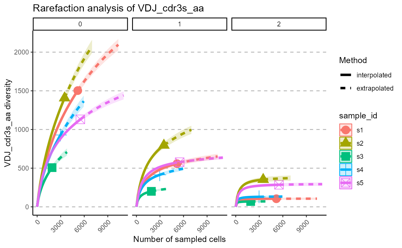
p[[2]]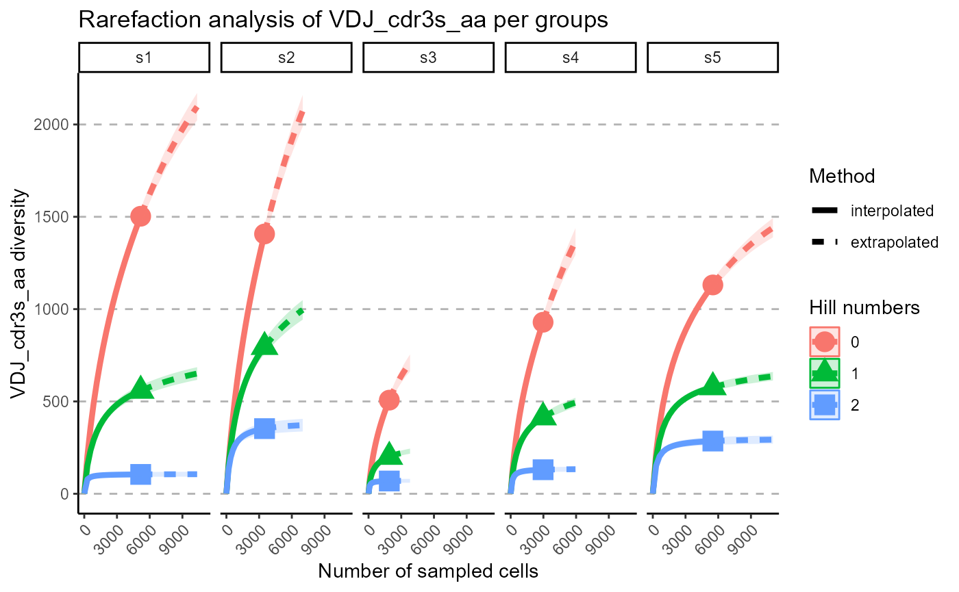
The output of VDJ_rarefaction is a list of two plots: the first plot includes the rarefaction curves of each sample across each Hill number, whereas the second has the Hill numbers in the same subplot, grouped by samples.
5.2 Selecting Hill numbers
We can select particular Hill numbers to be plotted via the hill.numbers parameter. 0 - species richness, 1 - Shannon diversity, 2 - Simpson diversity. For example, we chose to only rarefy the species richness in the following plots.
p <- VDJ_rarefaction(VDJ,
                feature.columns = 'VDJ_cdr3s_aa',
                grouping.column = 'sample_id',
                hill.numbers = 0)
## Warning in ggiNEXT.iNEXT(inext_object, type =
## rarefaction_type_dict[rarefaction.type], : invalid facet.var setting, the iNEXT
## object do not consist multiple orders.
p[[1]]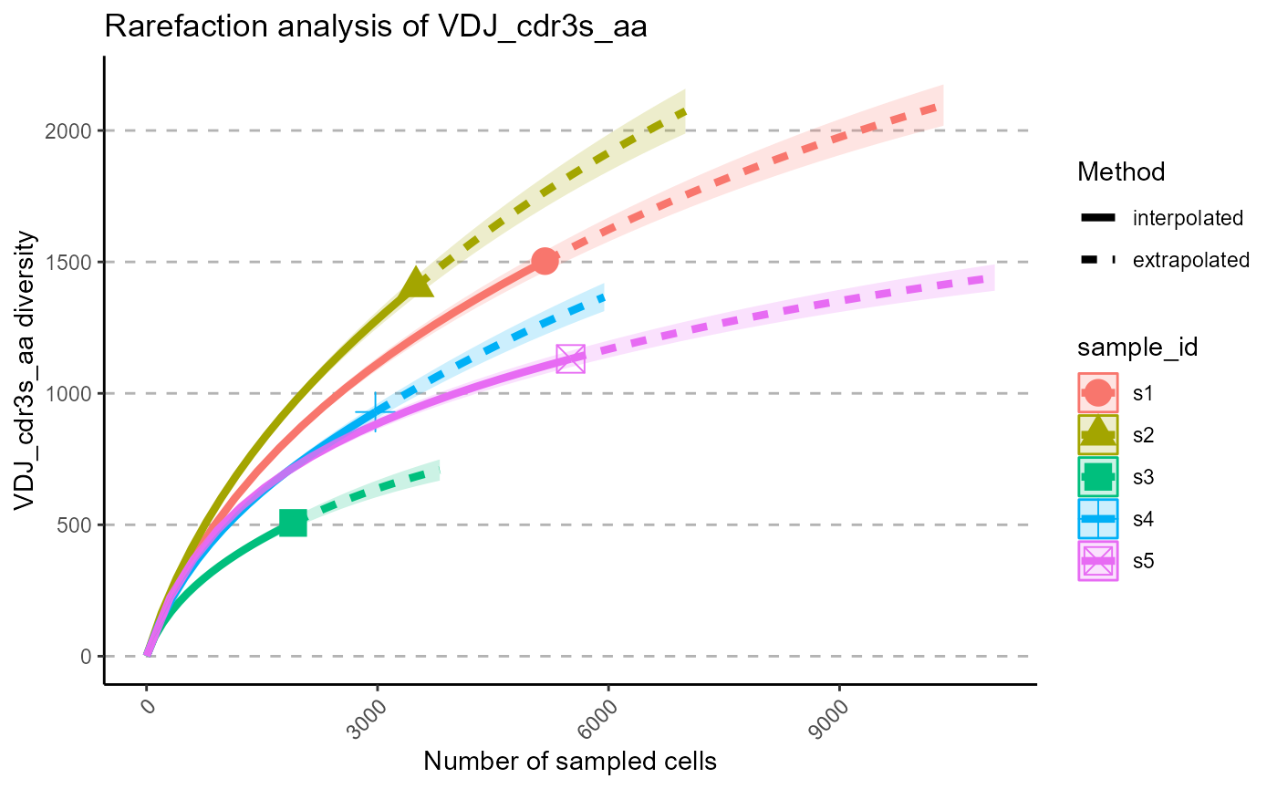
p[[2]]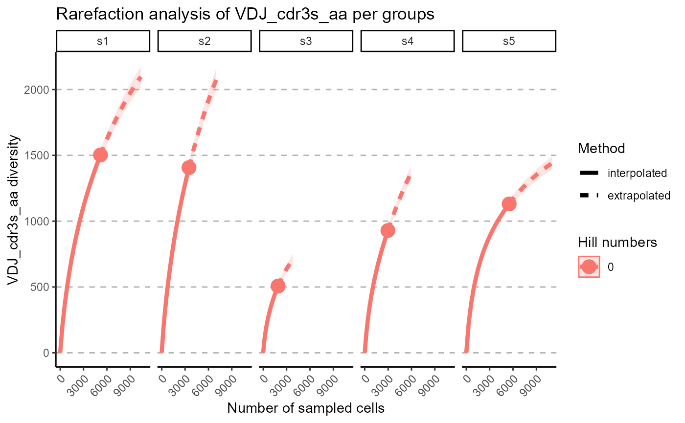
6. VDJ_ordination dimensionality reduction/ordination analysis
Ordination methods are a set of dimensionality reduction approaches used in community ecology for easier visualization of samples and/or species from an incidence matrix/ community data matrix (samples by species). Currently, the following dimensionality reduction algorithms are supported in VDJ_ordination: PCA (method = ‘pca’), t-SNE via the Rtsne R package (method = ‘tsne’), UMAP via the umap R package (method = ‘umap’), detrended correspondence analysis/DCA via the vegan package (method = ‘dca’) and PCOA/ Multidimensional scaling - MDS via the vegan package (method = ‘mds’).
6.1 Ordination methods/algorithms
We will showcase the sample ordination for the following methods: PCA, t-SNE, UMAP, and DCA.
#PCA dim reduction/ ordination
p1 <- VDJ_ordination(VDJ,
               feature.columns = 'VDJ_cdr3s_aa',
               grouping.column = 'sample_id',
               method = 'pca',
               reduction.level = 'groups')

#t-SNE dim reduction/ ordination
p2 <- VDJ_ordination(VDJ,
               feature.columns = 'VDJ_cdr3s_aa',
               grouping.column = 'sample_id',
               method = 'tsne',
               reduction.level = 'groups')

#UMAP dim reduction/ ordination
p3 <- VDJ_ordination(VDJ,
               feature.columns = 'VDJ_cdr3s_aa',
               grouping.column = 'sample_id',
               method = 'umap',
               reduction.level = 'groups')

#DCA dim reduction/ ordination
p4 <- VDJ_ordination(VDJ,
               feature.columns = 'VDJ_cdr3s_aa',
               grouping.column = 'sample_id',
               method = 'dca',
               reduction.level = 'groups')

cowplot::plot_grid(p1, p2, p3, p4)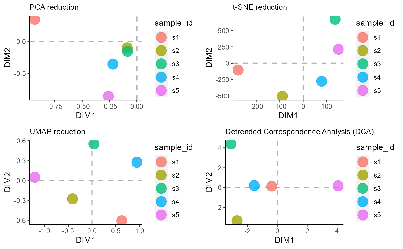
6.2 Ordination across groups
The reduction.level parameter controls whether dimensionality reduction will be performed across samples, features/sequences, or across both (resulting in a plot with both samples and shared features). For ordination across samples, use reduction.level = ‘groups’.
VDJ_ordination(VDJ,
               feature.columns = 'VDJ_cdr3s_aa',
               grouping.column = 'sample_id',
               method = 'mds',
               reduction.level = 'groups')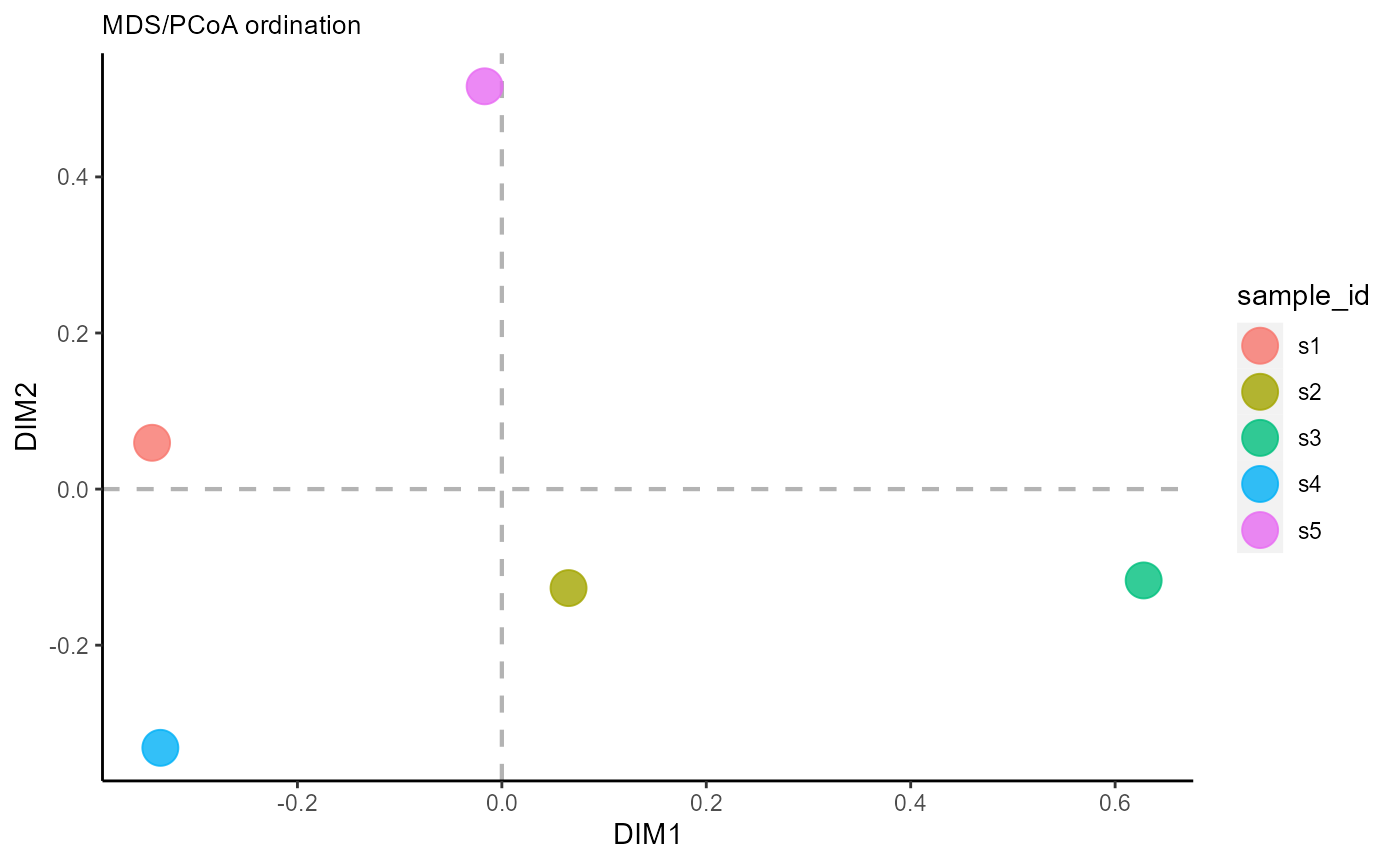
6.3 Ordination across features
For ordination across the CDRH3 incidence vectors, use reduction.level = ‘features’. Currently, custom point colors in the resulting graph are not available.
VDJ_ordination(VDJ,
               feature.columns = 'VDJ_cdr3s_aa',
               grouping.column = 'sample_id',
               method = 'mds',
               reduction.level = 'features')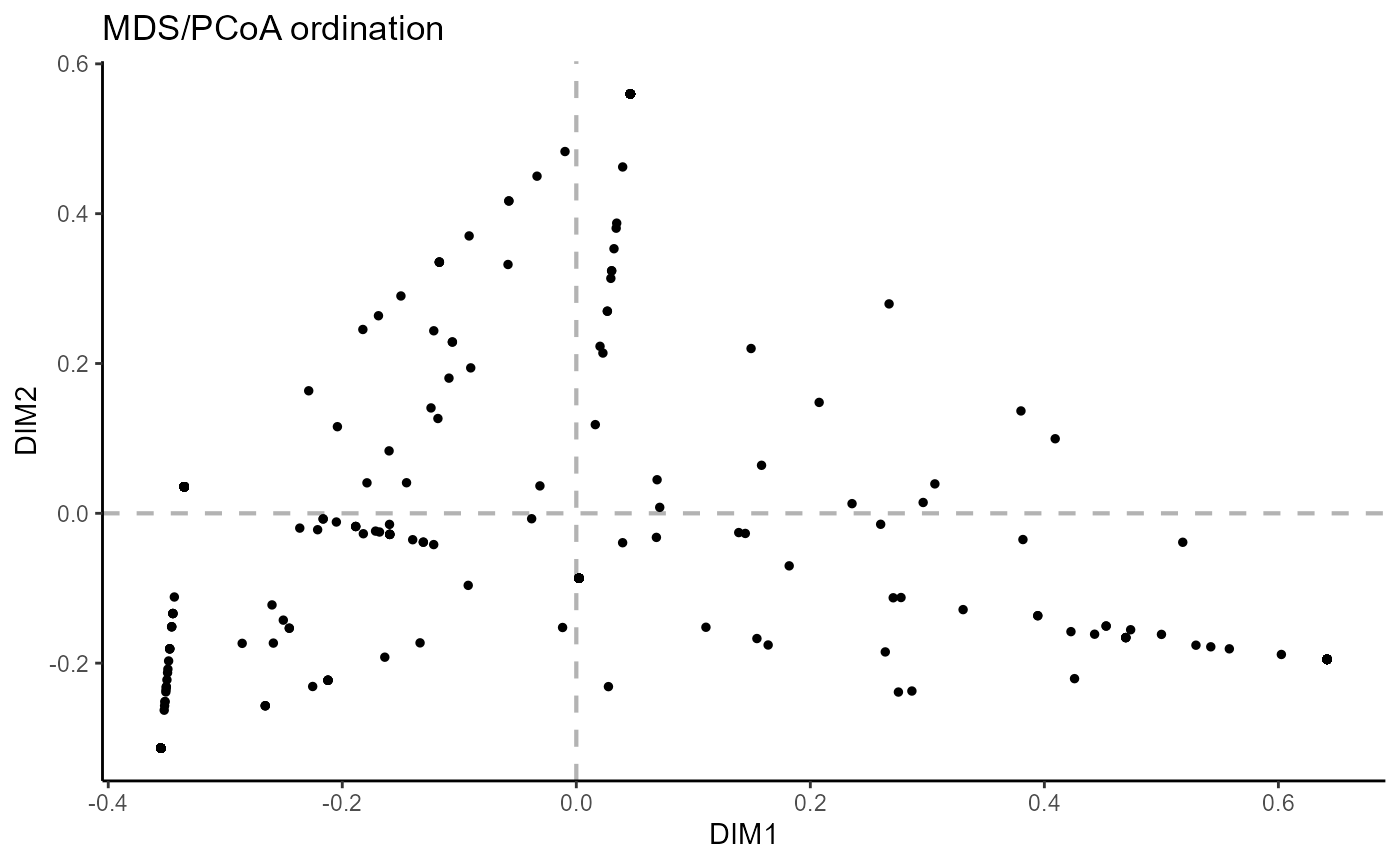
6.4 Ordination across both groups and samples
reduction.level = ‘both’ performs dimensionality reduction for both samples and features.
VDJ_ordination(VDJ,
               feature.columns = 'VDJ_cdr3s_aa',
               grouping.column = 'sample_id',
               method = 'mds',
               reduction.level = 'both')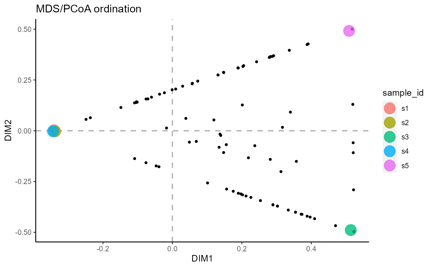
7. Version information
## R version 4.2.1 (2022-06-23 ucrt)
## Platform: x86_64-w64-mingw32/x64 (64-bit)
## Running under: Windows 10 x64 (build 19044)
##
## Matrix products: default
##
## locale:
## [1] LC_COLLATE=German_Germany.utf8  LC_CTYPE=German_Germany.utf8
## [3] LC_MONETARY=German_Germany.utf8 LC_NUMERIC=C
## [5] LC_TIME=German_Germany.utf8
##
## attached base packages:
## [1] stats     graphics  grDevices utils     datasets  methods   base
##
## other attached packages:
## [1] Platypus_3.4.1
##
## loaded via a namespace (and not attached):
##  [1] sass_0.4.2         tidyr_1.2.0        jsonlite_1.8.0     viridisLite_0.4.0
##  [5] splines_4.2.1      bslib_0.4.0        assertthat_0.2.1   askpass_1.1
##  [9] highr_0.9          yulab.utils_0.0.5  yaml_2.3.5         pillar_1.8.0
## [13] lattice_0.20-45    reticulate_1.25    glue_1.6.2         digest_0.6.29
## [17] colorspace_2.0-3   ggfun_0.0.6        cowplot_1.1.1      htmltools_0.5.3
## [21] Matrix_1.4-1       plyr_1.8.7         pkgconfig_2.0.3    purrr_0.3.4
## [25] patchwork_1.1.1    tidytree_0.3.9     scales_1.2.0       ggplotify_0.1.0
## [29] RSpectra_0.16-1    Rtsne_0.16         openssl_2.0.2      tibble_3.1.8
## [33] mgcv_1.8-40        generics_0.1.3     farver_2.1.1       ggplot2_3.3.6
## [37] ellipsis_0.3.2     cachem_1.0.6       umap_0.2.8.0       lazyeval_0.2.2
## [41] cli_3.3.0          magrittr_2.0.3     memoise_2.0.1      evaluate_0.15
## [45] fs_1.5.2           fansi_1.0.3        nlme_3.1-157       MASS_7.3-57
## [49] vegan_2.6-2        textshaping_0.3.6  tools_4.2.1        lifecycle_1.0.1
## [53] stringr_1.4.0      aplot_0.1.6        ggtree_3.4.1       munsell_0.5.0
## [57] cluster_2.1.3      compiler_4.2.1     pkgdown_2.0.6      jquerylib_0.1.4
## [61] gridGraphics_0.5-1 systemfonts_1.0.4  rlang_1.0.4        grid_4.2.1
## [65] ggridges_0.5.3     rstudioapi_0.13    labeling_0.4.2     rmarkdown_2.14
## [69] gtable_0.3.0       DBI_1.1.3          reshape2_1.4.4     iNEXT_2.0.20
## [73] R6_2.5.1           knitr_1.39         dplyr_1.0.9        fastmap_1.1.0
## [77] utf8_1.2.2         rprojroot_2.0.3    treeio_1.20.1      ragg_1.2.2
## [81] permute_0.9-7      desc_1.4.1         ape_5.6-2          stringi_1.7.8
## [85] parallel_4.2.1     Rcpp_1.0.9         png_0.1-7          vctrs_0.4.1
## [89] tidyselect_1.1.2   xfun_0.31